Excel has some magic formatting options. With conditional formatting I’ve created my own little calendar with highlighted current day / month / date. Full sample for download below this post.

The screenshot is from March 16, but you’ve already seen that 😉

Current day

In the header of the calendar I’ve set all days (1-31) The value of each column can be compared to the DAY function. With the conditional formatting of Excel I can highlight the current day.

Based on the cell value that is compared to the calculated current day Excel will apply special formatting to the current day.

Current month

The months are in the vertical header of the calendar. Only difference with the day is the use of abbreviated names in stead of numbers. That is where the INDEX function comes in. With the INDEX function Excel will return the contents of a certain ROW (and COLUMN) in an area.

' A3:A14 = the vertical header
' AH3 = the calculated current month
=INDEX(A3:A14;AH3)

Now apply a conditional formatting rule to the vertical header based on the cell value and the month is highlighted.

Current date

To highlight the current date in the calendar I use the CELL function. With that I can get the column and the row of each cell.

' $AH$2 = the current day
' $AH$3 = the current month
=AND($AH$2 = CELL("col";A1);$AH$3 = CELL("row";A1))

Important was the [reference] parameter of the CELL function. This is the relative location to get the information for. A1 means the current cell.

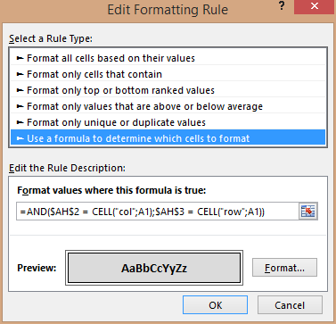
The conditional formatting is now based on a formula. Excel will evaluate the formula for each cell and highlight the cells that evaluate to TRUE.

References

Download Excel file with 2015 calendar